< Coursera Ordered Data Structures >
Binary Search Tree
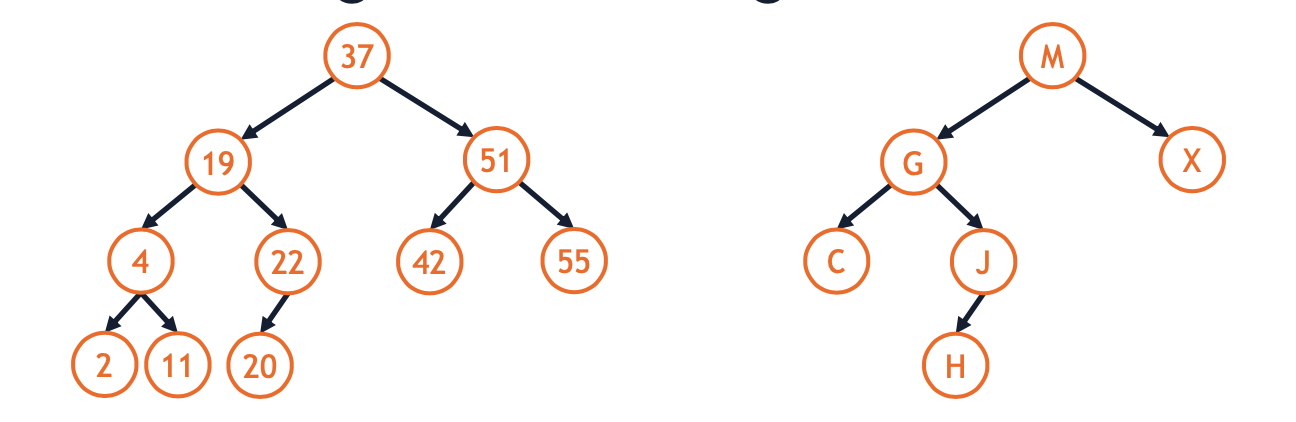
- A binary search tree (BST) is an ordered binary tree capable of being used as a search structure
- A binary tree is a BST if for every node in the tree:
- nodes in the left subtree are less than itself
- nodes in the right subtree are greater than itself
Dictionary
- A dictionary associates a key with data:
- your login email -> your profile data
- your phone number -> your phone record
- a website URL -> the webpage
- your street address -> your home
Dictionary ADT
find: finds the data associated with a key in the dictionaryinsert: adds a key/data pair to the dictionaryremove: removes a key from the dictionaryempty: returns true if the dictionary is empty
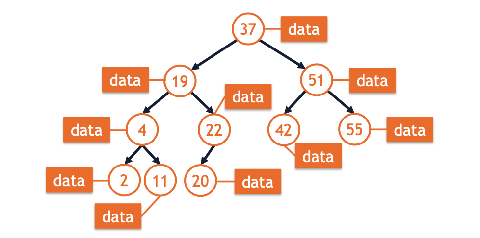
BST-Based Dictionary
- A BST used to implement a dictionary will store both a key and data at every node:
#pragma once

template <typename K, typename D>
class Dictionary {
  public:
    // Let the constructor just initialize the head pointer to null.
    Dictionary() : head_(nullptr) { }
    const D& find(const K& key);
    void insert(const K& key, const D& data);
    const D& remove(const K& key);

  private:
    class TreeNode {
      public:
        const K& key;
        const D& data;
        TreeNode* left;
        TreeNode* right;
        TreeNode(const K& key, const D& data)
          : key(key), data(data), left(nullptr), right(nullptr) { }
    };

    TreeNode *head_;
- So, all of these things are just like a tree that we were introduced to earlier, but now we’re going to do a dictionary class that implements a binary search tree, that’s going to allow us to make searches efficient.
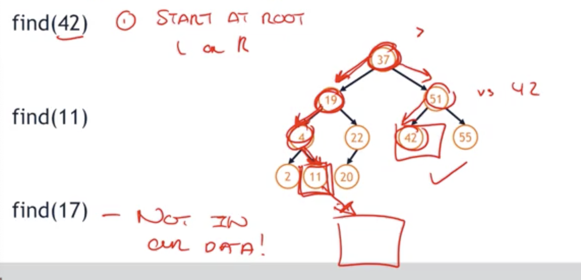
Example: Finding in a BST
-
find(42)
- Start at root : 42 > 37 => go right
- 42 < 51 => go left
=> go to the node, look at the left and right node and compare
-
find(11)
- 11 < 37 => go left
- 11 < 19 => go left
- 11 > 4 => go right
-
find(17)
- 17 < 37 => go left
- 17 < 19 => go left
- 17 > 4 => go right
- 17 > 11 => go right but there’s no node 11!
=> Once we’ve gone one path through the tree following the rules every step of the way, if we reach the end and we haven’t found the data, we know for a fact that that data is not in our data structure even though we haven’t searched the entire tree.
Runtime of BST:find
- So, as we move through this longest path, we’re taking a lot of steps looking through data, but notice we’re not looking through all of the data, this is not as bad as an array or a linked list where we have to travel over every single piece of data, here we only need to take one path through the tree.
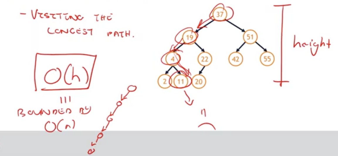
- Let’s think about worst-case outcome of fine
- visiting the longest path which has same height of tree’s height
O(h)is very worst case of time (h is height)- worst case’s path looks like just a linked list
- The very very very worst case is our tree looks like it linked lists it’s not a very complete tree, is a tree that simply has one long chain all the way to the left or all the way to the right, this one long chain is going to have a path-link that’s going to be equal to number of nodes in the tree and the height is going to be proportional to number of nodes in the tree.
template <typename K, typename D>
const D& Dictionary<K, D>::find(const K& key) {
  TreeNode*& node = _find(key, head_);
  if (node == nullptr) { throw std::runtime_error("error: key not found"); }
  return node->data;
}

template <typename K, typename D>
typename Dictionary<K, D>::TreeNode*& Dictionary<K, D>::_find(
  const K& key, TreeNode*& cur) const {
    if (cur == nullptr) { return cur; }
    else if (key == cur->key) { return cur; }
    else if (key < cur->key) { return _find(key, cur->left); }
    else { return _find(key, cur->right); }
}
- All we have to do is simply start at the root of the tree and traverse through the tree going left or right based on comparison of the value to my key and then once we found our data or found the end of the tree, we simply return that node being the data itself or a null pointer.
Insert into a BST
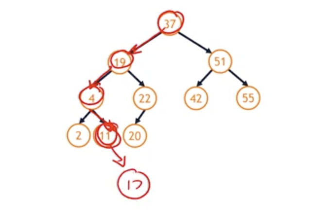
- insert(17)
- All we need to do is to find a location of the data that we’re inserting.
- 37 -> 19 -> 4 -> 11 -> inserting 17
- Now we can add 17!
- The insert algorithm is trivial because we’re able to use the fact the find algorithm returns a pointer by reference to the exact location where we need to insert at.
/**
* insert()
* Inserts `key` and associated `data` into the Dictionary.
*/
template <typename K, typename D>
void Dictionary<K, D>::insert(const K& key, const D& data) {
  TreeNode *& node = _find(key, head_); // find the location of the right place to insert
  node = new TreeNode(key, data);
}
Remove from a BST
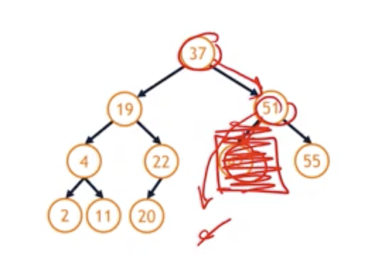
- remove(42)
- use
find()function - 37 -> 51 -> 42
- setting the node 42 to null
- use
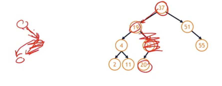
- Remove(22)
- 37 -> 19 -> 22
- We can’t simply remove 22 because we’ll lose the track of 20.
- But this again looks like a linked list, if we consider the fact that we just have nodes linked together like this, we know exactly how to repair this because we’ve repaired a linked list instead of simply deleting everything at this pointer and setting it equal to null, we delete the node and repair it by moving this pointer to the one child.
- One-child remove is easy case because it’s like case of linked list.
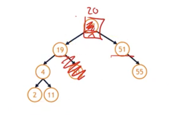
- Remove(37) - two child
- problem : 19 should be the root or 51 should be the root? And how can we repair this tree?
- The best candidate is probably going to be the node that is best suited to be at the root position in a tree that wouldn’t disturb anything else about the tree.
- The best node to replace 37 is going to be the node that is closest to 37, either less than it or greater than it. So 37 and 20, 20 is the best node in this left sub-tree to replace 37. So, imagine this is 20, and everything else remains the same. Given this element is now 20, 19, 4, 2, and 11 all sit on left-hand side, this looks good, 51 and 55 all sit on the right hand side.
In-Order Predecessor (IOP)
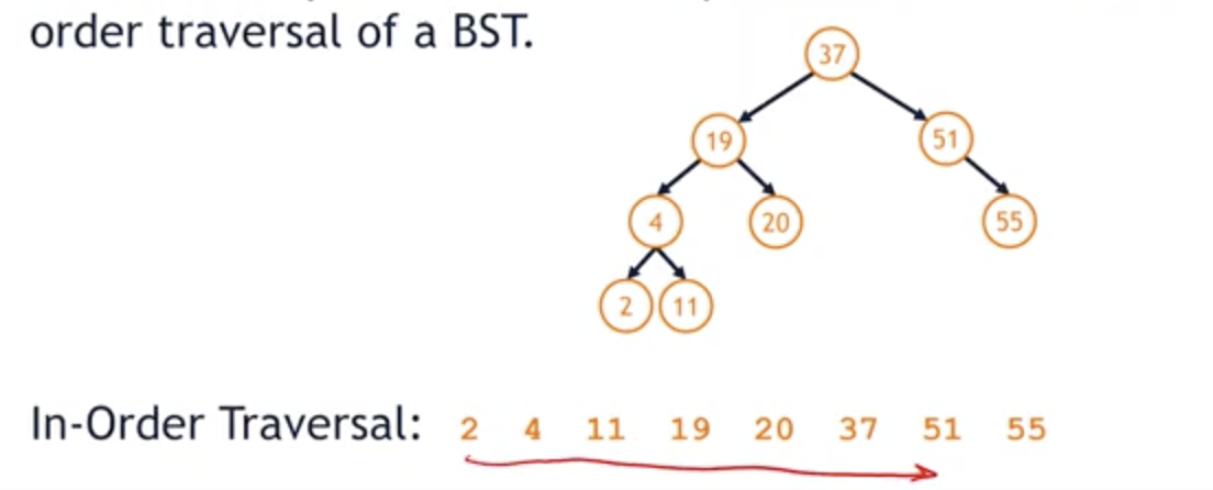
- The in-order predecessor is the previous node in an in-order traversal of a BST.
- We’ll say that we are going to replace the root of the tree with what we’re going to refer to as the in-order predecessor of a given node, or the IOP.
- The in-order predecessor of a node is going to be an in-order traversal of a binary search tree such that we choose the element that appears immediately before the route. (in-order traversal을 하다가 루트노드 직전에 마주치는 노드로 루트를 바꿈)
- So, the route is 37, so the in-order predecessor is going to be that element 20 when we do an in-order traversal.
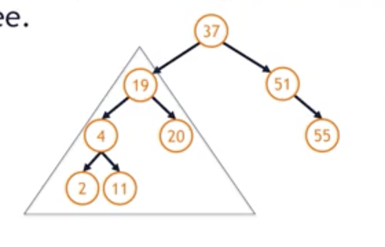
- Clever way to find IOP : the IOP of a node will always be the right-most node in the node's left sub-tree
BST::remove
Zero children: Simple, delete the nodeOne child: Simple, works like a linnked listTwo children:- Find the IOP of the node to be removed
- Swap with the IOP
- Remove the node in it’s new position which will either be a case of a one-child remove or a zero-child remove
=> We have this algorithm that some are recursively defined in the sense that we’re swapping something and then removing it using that same remove algorithm, but by doing that, we’re guaranteeing that the swap is going to be an easier case.
/**
* remove()
* Removes `key` from the Dictionary. Returns the associated data.
*/
template <typename K, typename D>
const D& Dictionary<K, D>::remove(const K& key) {
  TreeNode*& node = _find(key, head_);
  return _remove(node);
}

template <typename K, typename D>
const D & Dictionary<K, D>::_remove(TreeNode *& node){
  // Zero child remove:
  if(node->left == nullptr && node->right == nullptr){
    const D & data = node->data;
    delete(node);
    node = nullptr;
    return data;
  }
  // One-child (left) remove
  else if(node->left != nullptr && node->right == nullptr){
    const D & data = node->data;
    TreeNode *temp = node;
    node = node->left;
    delete(temp);
    return data;
  }
  // One-child (right) remove
  else if(node->left == nullptr && node->right != nullptr){
    const D & data = node->data;
    TreeNode *temp = node;
    node = node->right;
    delete(temp);
    return data;
  }
  // Two-child remove:
  else {
    // Find the IOP
    TreeNode *& iop = _iop( node->left );

    // Swawp the node to remove and the IOP
    _swap( node, iop );

    // Remove the new IOP node that was swapped
    return _remove( node );
  }
}
Binary Search Tree Analysis
- Binary Search Trees (BSTs) can take on many forms and structures, even containing the same data:
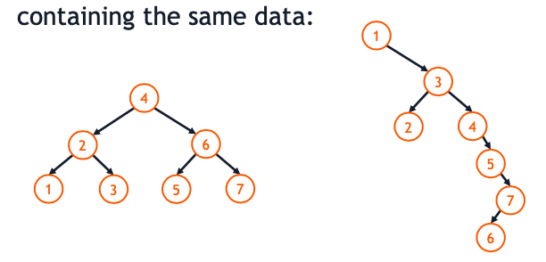
- Both of them are correct Binary Search Tree in a sense that all nodes on the right side have bigger data than it’s mother node, and on the left side have smaller data, but they have very different structure.
BST Forms
- Both trees contain the values {1, 2, 3, 4, 5, 6, 7}:
- Insert Order: 4, 2, 3, 6, 7, 1, 5
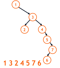
-
Insert Order: 1, 3, 2, 4, 5, 7, 6
-
So, what is efficient BST? What is the best case and what is the worst case?
Puzzle
- How many possible ways can we insert the same data into a BST?
- Let’s say, we have numbers 1 2 3 4 5 6 7
- Let’s say, we insert 5 as a root
- Now, we have choice of 6 other nodes to insert second. We can choose 2
- Now we have choice of 5 … next we have choice of 4.. 3.. 2.. 1
- => number of possible way to insert these 7 numbers = 7 * 6 * 5 * 4 * 3 * 2 * 1 => 7!
- => n!
| Operation | BST Average Case :) | BST Worst Case :( | Sorted Array | Sorted List |
|---|---|---|---|---|
| find | O(lg(n)) | O(n) | O(lg(n)) | O(n) |
| insert | O(lg(n)) | O(n) | O(n) | O(n) |
| remove | O(lg(n)) | O(n) | O(n) | O(n) |
- BST Worst Case
- Find :
O(n)- It is a tree with the structure of linked list, linked as a one line
- It shoud visit all nodes to find the right data, because in linked list, we can’t skip any element data.
- Insert & Remove :
O(n)- Remember that all of our operations depend upon find. So when we’re finding an element in a binary search tree, we insert it by just adding one more line of code. We remove it by just considering four particular cases that in itself only call find. So we find for a binary search tree the running time of find is going to be the running time of both insert and remove, because insert and remove only do constant time operations after finding the element.
- Find :
- Sorted List
- Find :
O(n)- It also takes O(n) because it’s a ‘List’. We can’t skip any element data.
- Insert & Remove :
O(n)- We should find the right place first, which takes O(n) so inserting and removing also take O(n).
- Find :
- Sorted Array
- Find :
O(lg(n))- We can jump right to the middle of the array, and if it’s not the data that we’re looking for, we can go left if it’s less than the middle data, or go right if it’s greater, because it’s sorted!
- Insert & Remove :
O(n)- sorted array, we’ve discussed the idea that an array has to be contiguous memory. So if we insert and we move from an array, this is going to be O(n) time.
- Find :
- BST Average Case
- Find :
O(lg(n))- The average BST case is a tree that has half of its elements on the right and half of its elements on the left.
- Insert & Remove :
O(lg(n))- Remember that all of our operations depend upon find. So when we’re finding an element in a binary search tree, we insert it by just adding one more line of code. We remove it by just considering four particular cases that in itself only call find. So we find for a binary search tree the running time of find is going to be the running time of both insert and remove, because insert and remove only do constant time operations after finding the element.
- Find :
- => The best algorithm which takes O(lg(n)) at all operation types, find, insert, and remove is BST Average Case.
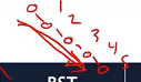
Height Balance Factor
- The height balance factor (b) of a node is the difference in height between its two subtrees
-
b = height(TR) - h(TL)
-
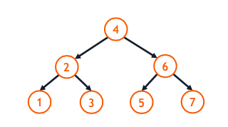
Left tree : 1 -1 = 0 => this tree is perfectly balanced
-
Right Tree : 4 - (-1) = 5 => this tree is heavily biased to the right
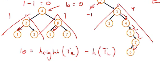
Balanced BST
-
A balanced BST is a BST where every node’s balance factor has a magnitude of 0 or 1:
-
This means that all balance factor of all subtrees have either -1, 0 or 1.
- Left Tree : every subtrees have balance factor of 0, so it’s balanced BST.
- Right Tree :
- node 6 : b = 0
- node 7 : b = -1
- node 5 : b = 2
- node 4 : b = 3
- node 3 : b = 3
- node 1 : b = 5
Summary of BST Analysis
- There are n! different ways to create BSTs with the same data.
- The worst-case BST will have a height proportional to the number of nodes.
- An average BST(relatively balanced tree) will have a height proportional to the logarithm of the number of nodes.
- Using a height balance factor, we can formalize if a given BST is balance.